Arc Catalog and ArcMap Basics

Exploring ArcMap and ArcCatalog

ArcMap

• Allows you to work with all of your geographic data in maps, regardless of format or location of the data (ie., shapefile, jpg, text file)
• Allows you to quickly assemble a map from predefined layers, or add data from coverages, shapefiles, geodatabases, grids, TINs, images, and tables of coordinates or addresses

ArcCatalog

• Browse, organize, and document data
• Designed to work with ArcMap
• Drag and drop data files from ArcCatalog onto an existing map in ArcMap

ArcToolbox

• Accessible through both ArcMap and ArcCatalog
• Contains tools for performing sophisticated geoprocessing operations on your data

Exploring Data in ArcCatalog

1. Open ArcCatalog (Start, All Programs, ArcGIS, ArcCatalog)

2. Catalog tree(TOC) – Branches for each local hard drive. Branches for other ArcGIS connections can be added by clicking the Tools menu, then choose Options, then click any checkboxes next to the branches you want to add to the catalog tree.

3. You can also create new branches (connections) in the tree to make it easier to connect to your data.

4. Next, you will make a connection to the folder that contains the Exercise data

5. This new branch in the catalog tree will remain until you disconnect it.

6. On the Toolbar, click the Connect to Folder button.

7. Browse and connect to the C:/temp/ArcGIS_Exercuise folder.

8. Click to highlight the Exercises folder and click OK.

9. The new connection shows up as a branch in the Catalog tree..

10. You can now explore the data in the folder you have added.

11. Click to highlight the C:/temp/ArcGIS_Exercises folder to view its contents on the right-hand side of the ArcCatalog window.

12. Click the plus sign (or double-click) to expand the connection in the Catalog tree.

13. This branch of the tree contains a folder called ‘data’ and several map documents (with a .mxd extension).

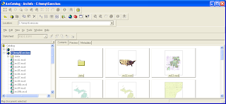
14. Click the plus sign to expand the data folder to view its contents in the tree. Highlight the data folder to view its contents in the right-hand side display window (in the “Contents” tab).

15. ArcCatalog recognizes many different types of files. In the data folder, we have more folders (buildings, michigan), a personal geodatabase folder (Umich.mdb), tables (campusalcohol.dbf), shapefiles (cities.shp), a layer file (Roads.lyr), and more.

16. Each of the map documents (ie., ex 02 .mxd) in the Exercises folder are general purpose maps that we will be using in the upcoming exercises, which reference the data files in the data folder.

17. Having this connection set in ArcCatalog will make it easy for us to navigate the data and open map documents .

18. Viewing thumbnail sketches – useful for selecting a particular map or data file from many different ones available

19. Click to Highlight the C:/temp/ArcGIS_ Exercises connection in the Catalog tree.

20. Click the Thumbnails button on the Standard toolbar.

21. Look at the thumbnail sketches for the various map documents.

22. Let’s open the ex02.mxd map document to view it in ArcMap.

23. To do this, double-click ex02.mxd in the Catalog tree. This starts ArcMap

and opens the map document.

The ex02.mxd map document displays data from the data folder

• The streetpaths layer is a line feature class contained within the Umich.mdb personal geodatabase, which represents streets on campus
• The umbuildings layer is a polygon feature class also within the Umich.mdb folder, which represents buildings on campus
• The um layer is a polygon feature class also within the Umich.mdb folder, which represents UM property
• The Roads layer (top layer in the ArcMap table of contents), which is currently turned off, is neither a feature class nor a shapefile. It is a layer file (.lyr), which references the streetpaths feature class in the Umich.mdb folder. A .lyr is a set of rules for displaying and working with datasets including symbol assignments, classifications, labeling rules, etc. In this case, the Roads.lyr file symbolizes the streetpaths feature class with different color/size lines for the different street/road types.
• To view the Roads layer, turn it on by checking the box next to Roads in the table of contents.

Connecting to GIS Servers:

1. The Geography Network portal

-The main theme of the Geography Network is the sharing of geographic information

-As more people begin to see the value of using GIS to structure their organization and solve their problems, the need for easy access to geographic information continues to rise

-The Geography Network is a global network of geographic information users and providers. It delivers geographic content over the internet to user browsers and desktops. Content may be provided in the form of raw data, maps, or more advanced services, for example, lifestyle mapping, flood risk mapping, address geocoding, and network routing

-The Geography Network is also a global community of government and commercial users, data publishers, and service providers, who contribute to making geographic content more widely available.

25. Open ArcCatalog (if necessary)

26. Scroll down and expand the ‘GIS Servers’ folder

27. Double-click ‘Add ArcIMS Server’

28. In the ‘URL Server’ box, type ‘www.geographynetwork.com’ and click ‘ok’

Expand the new ‘www.geographynetwork.com’ connection

29. View the available services (preview, content, metadata)

30. Start ArcMap (click on the Launch ArcMap button)

31. Click and drag a service from the Catalog tree into the ArcMap display window

Chapter 1

Chapter 3

Chapter--3

Chapter--4

Chapter 5

Chapter 5

Chapter 6

Chapter 7

Chapter 8

Importing Data into ERDAS Imagine

Any image file to be worked in ERDAS is to be converted into Image(*.img) format. Observe the video to convert any type of file to .img format. Here in the below example I've used JPEG image, similarly ERDAS supports many formats to be used.

• Go to ERDAS Imagine
• Click on Import/Export Module
• Specify the input format from the drop down box
• Browse the input file
• Give the destination folder for Output file and click on ok
• After the process bar completes click on Done.

ERDAS- GeoRectification of Topo Sheet

Geometric Correction or Geo-Rectification of a Topo graphical sheet

Topographic maps are also commonly called contour maps or topo maps, are large-scale detail and quantitative representation of relief usually called contour lines in modern mapping.

Georeferencing

Georeferencing refers to the process of assigning map coordinates to image data. The image data may already be projected onto the desired plane, but not yet referenced to the proper coordinate system. Rectification, by definition, involves georeferencing, since all map projection systems are associated with map coordinates. Image-to-image registration involves georeferencing only if the reference image is already georeferenced.

Georeferencing, by itself, involves changing only the map coordinate information in the image file. The grid of the image does not change.Geocoded data are images that have been rectified to a particular map projection and pixel size, and usually have had radiometric corrections applied. It is possible to purchase image data that is already geocoded. Geocoded data should be rectified only if they must conform to a different projection system or be registered to other rectified data.

Geometric Correction is the method of applying GCPs(Ground Control Points) to the image and project. When the image is Geometrically corrected one can measure distances and calculate areas very accurately.

Projection is the transformation of a three dimensional body(such as spherical Earth) to a two dimensional plane surface(paper ).All map projections distort the surface in some fashion. Depending on the purpose of the map, some distortions are acceptable and others are not; therefore different map projections exist in order to preserve some properties of the sphere-like body at the expense of other properties.

So a particular type of projection is choosen depending upon the geographical location of the area to be mapped.

Steps to achieve Geometric Correction in ERDAS

Basic Procedure:

• Display files
• Start Geometri correction tool
• record Geometric(ground) Control Points(C+GCPs)
• resample the image
• Verify

Begin by opening the file which you wish to georegister and display it and "fit" it in a viewer. As your mouse moves within the display window note that the coordinates displayed in the lower left of the viewer are in "row" and "column".

• Start the Geometric Correction tool from the viewer displaying the file to be retified.
• Select RASTER > Geometric Correction from the viewer's menu bar and Polynomial from the dialog box.

• Each of these geometric models relate to specialized tasks. The polynomial model has the most general application.

Two dialogs boxes will appear. The Geo Correction Tool menu will be used now.

• The first one is Geo Correction Tools Window and the other is Polynomial model properties
• From the Polynomial model properties click on Projection Tab-->click on Add/Change projection.
• Select Datum--> Geographic Lat/Long
• Spreriod--> Everest 1956
• Datum name--> India Nepal

Click on GCP tool Reference Setup from the Polynomial model properties. You would observe the following dialog box:

• Select the option Keyboard Only. This option differs when you are Georectifying Image/Topo sheet from an existing Geometrically corrected Image/Topo sheet.
• Click on Ok

You are now ready to begin assigning real world coordinates to the non-geographic registered image.

• First, each viewer now has it's own "zoom" window above it. The zoom window display that part of the image which is inside the "box" (some time called the link box). The Ground Control Points (GCPs) are the small targets which are place on the image using the GCP tool .As you observer there are two viewers , one in which the image to be rectified is displayed and in the other a magnified part of the image is displayed.
• In the Viewer1 you would observe a magnifier box pointing to some area and the respective area is visible in the Viewer2 at a best zoom level.
• Now adjust the Maginifer box in the viewer to the top left corner of the topo sheet where you can see a cross hair mark having coordinates.
• From the GCP tool bar, select GCP tool and click on the cross hair in the Viewer1(Top Left Corner).
• As soon as you click on the viewer paper coordinates are added to the GCP control. You have to manually add the Geographic coordinates to the control, i.e, longitude and Latitude.

Note: In ERDAS Imagine you have to first add Longitude and later Latitude.

You need not convert Geographic coordinates whhich are in Degree Min Sec to Decimal coordinates.

Ex:17045'50"

Add them as 17 45 50 in the table provided X and Y Reference, they will be added as Decimal Coordinates.

• Repeat this for Top-Right, Bottom Left and Bottom Right Corners in the Topo sheet(Anti clock wise direction)

Save the Input from the table file menu

• Our next task is to resample the image . Resampling is the process of calculatin the values for the rectified image and creating the new file. All of the raster data layers (all bands) in the source file are resampled. The best known algorithms for resampling are Nearest Neighborhood, Bilinear Interpolation, and Cubic Convolution. We'll use the Nearest Neighborhood algorithm.
• Click on the resampling icon from the Geo Correction Tool Menu . The resample dialog opens. Enter a file name for the output (know where on the drive you will put the file) - select the Nearest Neighborhood resampling method - click to exclude zero file values in the statistics.

A job status dialog opens to let you know when the processes is complete.

• Verify the rectification by displaying the new image in a viewer and Geo. Link the reference image with the new image and use an Inquire Cursor to check that they are georegistered to each other.

Find the below video file recorded while performing Geometric Correction in ERDAS for a Topo sheet

------------------